Histogram sampling
Given an unknown probability distribution and sufficient data sampled from it, it is possible to sample additional data approximating the unknown distribution with a histogram. Let’s pretend we have some data, which are sampled from an unknown distribution:
import numpy as np
import matplotlib.pyplot as plt

np.random.seed(42)
data = np.random.rayleigh(size=100) ## unknown distribution
We can generate a histogram with an arbitrary number of bins. The more are the bins, the most precise will be the sampling, but most of the bins should contain a sufficient number of counts to be statistically significant. As a rule of thumb, I reduce the number of bins until the averaged populated bins have at least 5 elements.
bins = np.linspace(0, 5, 20)
hist, _ = np.histogram(data, bins=bins)
To sample from this histogram it is sufficient to calculate its cumulative distribution, extract a random number from a uniform distribution between 0 and 1 and finally find the index of the cumulative distribution where the random number should be inserted to keep the cumulative distribution sorted. The sampled number from the histogram will be the histogram bin corresponding to this histogram. To achieve this we can use the np.cumsum to calculate the cumulative distribution, the np.random.rand function to extract 1000 random number sampled from a uniform distribution, and the np.searchsorted function to find the index position of where these 1000 number should be inserted to preserve the ordering:
bin_midpoints = (bins[:-1] + bins[1:])/2
cdf = np.cumsum(hist)
cdf = cdf / cdf[-1]

values = np.random.rand(1000)
value_bins = np.searchsorted(cdf, values)
random_from_cdf = bin_midpoints[value_bins]
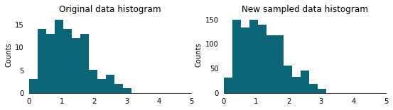
We can now plot the original (on the left) together with the histogram of the new sampled data random_from_cdf:
fig, (ax0, ax1) = plt.subplots(1, 2, figsize=(9, 3))
ax0.hist(data, bins=bins)
ax1.hist(random_from_cdf, bins=bins)

for ax in (ax0, ax1):
    ax.set(xlim=(0,5), ylabel='Counts')
    ax.tick_params(axis='x', color='none')
    ax.tick_params(axis='y', color='none')
    [ax.spines[d].set_visible(False) for d in ('top', 'left', 'right')]
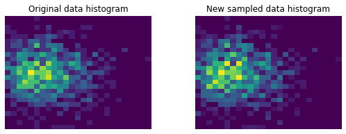
Histogram sampling in 2D
In two dimension the concept is the same, the only trick is to flatten the indexes when calculating the cumulative distribution:
np.random.seed(42)
BIN_COUNT = 25

data = np.column_stack((np.random.rayleigh(scale=30, size=1000),
                        np.random.normal(scale=15, size=1000)))
x, y = data.T

hist, x_bins, y_bins = np.histogram2d(x, y, bins=(BIN_COUNT, BIN_COUNT))
x_bin_midpoints = (x_bins[:-1] + x_bins[1:])/2
y_bin_midpoints = (y_bins[:-1] + y_bins[1:])/2

cdf = np.cumsum(hist.flatten())
cdf = cdf / cdf[-1]

values = np.random.rand(10000)
value_bins = np.searchsorted(cdf, values)
x_idx, y_idx = np.unravel_index(value_bins,
                                (len(x_bin_midpoints),
                                 len(y_bin_midpoints)))
random_from_cdf = np.column_stack((x_bin_midpoints[x_idx],
                                   y_bin_midpoints[y_idx]))
new_x, new_y = random_from_cdf.T


fig, axs = plt.subplots(1, 2, figsize=(9, 3))

axs[0].hist2d(x, y, bins=(BIN_COUNT, BIN_COUNT))
axs[0].set_title('Original data histogram')
axs[1].hist2d(new_x, new_y, bins=(BIN_COUNT, BIN_COUNT))
axs[1].set_title('New sampled data histogram')
for ax in axs:
    ax.set(aspect='equal')
    ax.set_axis_off()