ODE: quarter car model solver with scipy

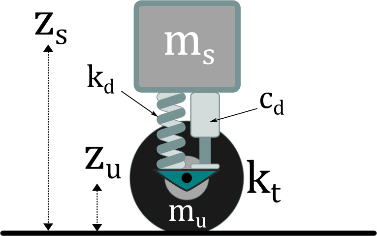
Here we show how one can use scipy to solve a simple differential equation. We use the so-called quarter car model as an example. This simple model describes the motion of a mass connected to a deformable wheel through a dumper-spring system. As shown in the scheme below, the components of the system are the following:
- Suspended mass: mass =
ms, and hight =zs - Tire: mass =
m_u(unsuspended), hight =zu, and elastic coefficient =kt - Dumper-spring system: dumping coefficient =
cd, and elastic coefficient =kd
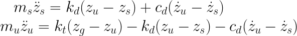
The equations of motions to solve are the following:
In python we need to create a function that takes as inputs:
t: the time stepy: the list of variables that will be integrated (position of the wheel and the suspended mass, and their derivative of positions in this example)- other constants and parameters
The function needs to return the derivative of the variables contained in y (the first and second derivative of the positions).
def quarter_car(t, y, ms, mu, kd, kt, cd, road_function):
    zs, vs, zu, vu = y
    zp = road_function(t)

    d1_zs = vs
    d2_zs = (kd*(zu-zs) + cd*(vu-vs))/ms

    d1_zu = vu
    d2_zu = (-kd*(zu-zs)-cd*(vu-vs)+kt*(zp-zu))/mu

    dydt = [d1_zs, d2_zs, d1_zu, d2_zu]
    return dydt
Code
To solve the equation using python we first need to import the following libraries. Note that the gaussian filter and interpolation are necessary only within this example and will be used to generate a random road profile.
from scipy.integrate import solve_ivp
import numpy as np
import matplotlib.pyplot as plt
import pandas as pd
from scipy.interpolate import interp1d
from scipy.ndimage.filters import gaussian_filter
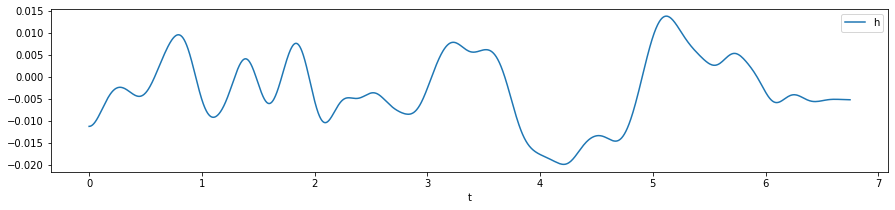
We now generate a random road profile:
profile_length = 150 #m
resolution = 0.005 #m
speed = 80 #Km/h
km_h_to_m_s = 1/3.6
amplitude = 0.5
sigma_gaussian_filter = 500

np.random.seed(41)
profile = pd.DataFrame(dict(
    pc = np.arange(0, profile_length, resolution),
    h = gaussian_filter(np.random.uniform(-amplitude, amplitude, size=int(profile_length/resolution)), sigma_gaussian_filter)
  ))
profile['t'] = profile['pc']/(speed*km_h_to_m_s)
profile.plot(x='t', y='h', figsize=(15,3));
We define the road profile function and the equations of motion:
def road_function(t):
    return interp1d(profile.t.values, profile.h.values)(t)


def quarter_car(t, y, ms, mu, kd, kt, cd, road_function):
    zs, vs, zu, vu = y
    zp = road_function(t)

    d1_zs = vs
    d2_zs = (kd*(zu-zs) + cd*(vu-vs))/ms

    d1_zu = vu
    d2_zu = (-kd*(zu-zs)-cd*(vu-vs)+kt*(zp-zu))/mu

    dydt = [d1_zs, d2_zs, d1_zu, d2_zu]
    return dydt
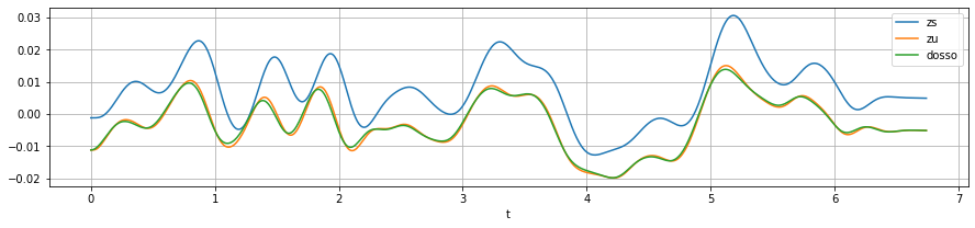
We finally use scipy to solve the equations and plot the results. The generated array sol.y will contain the positions and their first derivatives. Here, since we are interested in plotting only the position of the wheel and suspended mass we will use sol.y[0,:] and sol.y[2,:].
y0 = [road_function(0),0,road_function(0),0]
dt = 0.01

tmin = profile.t.min()
tmax = profile.t.max()
xmin = profile.pc.min()
xmax = profile.pc.max()

t = np.arange(tmin, tmax, dt)

kd = 20000
kt = 200000
cd = 2000
ms = 200
mu = 50

sol = solve_ivp(quarter_car, (tmin, tmax), y0, args=(ms, mu, kd, kt, cd, road_function), t_eval=t)

fig, ax = plt.subplots(1, figsize=(15, 3))
plt.plot(t, sol.y[0,:]+0.01,label='zs')
plt.plot(t, sol.y[2,:],label='zu')

plt.plot(t, road_function(t) ,label='dosso')
plt.legend(loc='best')
plt.xlabel('t')
plt.grid()
plt.show()