Bayesian optimization
Why Bayesian optimization
Bayesian optimization can be used for the global optimization of black-box function with no need to compute derivatives. In particular it can be exploited to efficiently optimize the hyper-parameters defining a neural network model and its training. Since the training of the NN can be very time consuming, it is important to explore the hyper-parameters space wisely. Solution like grid search or random search can be extremely costly and may not be feasible. Bayesian optimization is often a much better option, since it takes into account all the previously tested configurations to select the optimal next point to test, choosing the one that maximize the expected information gain.
Bayesian optimization in code
NB The code used to generate all the plots can be found here.
Lets give a look at how Bayesian optimization works in practice by using this python library by Fernando Nogueira.
We start by defining our black-box function, which will be completely unknown to the algorithm:
import numpy as np
import matplotlib.pyplot as plt

def black(x, y):
    sine_2d = np.sin(x*y*0.002)
    gaussian_2d = np.exp(-(x-50)**2/2000 -(y-70)**2/2000)*2
    return sine_2d + gaussian_2d + np.random.random(x.shape)/3

yy, xx = np.mgrid[0:100, 0:150]
zz = black(xx, yy)

plt.imshow(zz, origin=[0,0])
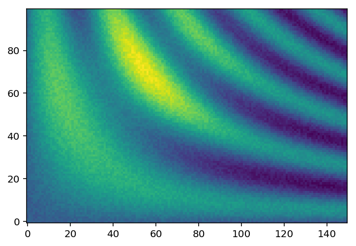
Our goal is to find the maximum of this function (most yellow region) by probing the function the least number of times. Lets set up the optimizer:
optimizer = BayesianOptimization(
    f=black,
    pbounds={'x': (0, 150), 'y': (0, 100)},
    verbose=2,
    random_state=30)

utility = UtilityFunction(kind="ei", xi=0.0, kappa=None)
The utility function defines the criteria to follow in order to pick the next point to probe. In this case we used ei which stands for Expected improvement. Lets run the optimization algorithm and see what happens:
for index in range(100):
    next_point_to_probe = optimizer.suggest(utility)
    target = black(**next_point_to_probe)
    optimizer.register(params=next_point_to_probe, target=target)
    # plot the result of the optimizer ...
 The black cross shows the current point being tested by the algorithm, the white dots represent all the previously tested point. The red dot shows the best point tested so far. The goal of the algorithm is to place the red dot on top of the most yellow region as fast as possible, without getting stuck in local maxima.
On the top left panel we plot our black-box function, which represents the ground truth we aim for. On the top right panel we plot the current best prediction of the function given the previously probed points (white dots). As we can see, the more point are acquired, the more faithful to the real black-box function is our prediction.
On the bottom left panel we plot the variance, which quantifies the uncertainty of our model in the parameter space. In the blue regions the variance is low, meaning that we are more confident about the goodness of our model. On the other hand, yellow regions correspond to high variance, i.e. high uncertainty regions. The bottom right panel shows the square difference between the ground truth and our prediction. We notice how the model is much more accurate to describe the black-box function (blue regions) where we tested the function the most.
The optimization algorithm which provides the next point to be probed can be chosen to be more exploitative or more explorative. In the former case the algorithm will be more greedy, trying to spot the maxima as fast as possible. This means that it will more likely explore regions close by the best optima previously find, but it also mean that it is more prone to get stuck into local maxima. On the other hand, the latter approach, is more conservative and probes the parameter space more evenly. It will more likely explore region of high uncertainty (yellow in the bottom left panel) in order to reduce the risk of missing the global maxima of the parameter space. A balance between exploration and exploitation is required and must be carefully considered: high exploitation can converge much faster, but it can converge to the wrong maxima. A good compromise can be starting the research with an exploratory mindset and then switch to exploitative after some iterations.
An example of highly explorative algorithm is the following:
# upper confidence bound
utility = UtilityFunction(kind="ucb", kappa=25., xi=None)

As we can see, the parameter space is explored much more evenly, drastically reducing the risk of getting stuck into local maxima, but the convergence is much slower. Notice how the next point to probe is often chosen as the one having the higher estimated variance.
On the other hand, an example of highly explorative algorithm is the following:
# probability of improvement
utility = UtilityFunction(kind="poi", xi=0.5, kappa=None)
 The algorithm is now greedy, and try to find the maxima as fast as possible. Notice how it explore regions very close to the last maxima found. We can clearly see the risk of being too greedy: within the initial steps it almost got stuck on the left local maxima.