Multi-Armed Bandit
In the k-armed bandit framework, the goal is to find the optimal action (between k actions), i.e. the one which maximizes a given reward. The player can perform any action and will receive a reward as a consequence. To find the best action to take, the player must balance exploration and exploitation. The former consists of testing all the actions to gain confidence about the reward they produce. The latter consists of performing actions which produce the highest expected reward.
10-armed bandit
Following the Richard S. Sutton and Andrew G. Barto book we create a testbed for the k-armed bandit problem as follow: we define 10 possible actions, each corresponding to a given reward probability distribution, i.e., when we perform a given action, we receive a reward sampled from the corresponding probability distribution. The probability distributions are defined as a normal distribution with variance 1 and mean different for each action. The mean on the distributions is also obtained randomly by sampling again from a normal distribution with zero mean and variance 1. Here’s an example of the ten reward distribution corresponding to the ten actions:
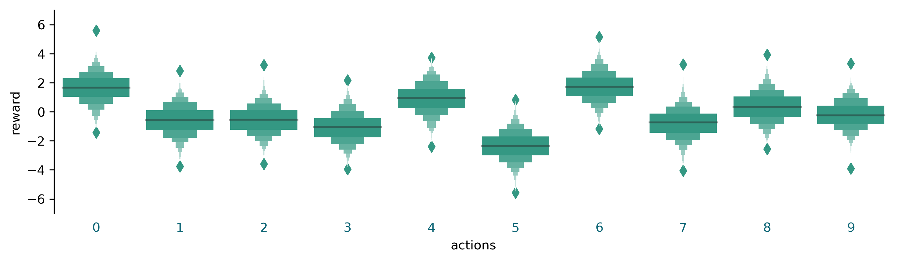
Here’s the code to produce the plot:
import numpy as np
import pandas as pd
import matplotlib.pyplot as plt
import seaborn as sns
%matplotlib inline

np.random.seed(1)
qs = np.random.normal(loc=0, scale=1, size=(10))
d = np.array([np.random.normal(loc=qs[a], scale=1, size=1000) for a in range(10)])
df = pd.DataFrame(d.T).melt(var_name='actions', value_name='reward')

fig, ax = plt.subplots(1, figsize=(10, 3))
sns.boxenplot(x='actions', y='reward', data=df,  ax=ax, color='#23a98c')
[ax.spines[pos].set_visible(False) for pos in ('right', 'bottom', 'top')];
[mt.set_color('#0c6575') for mt in ax.get_xmajorticklabels()];
[tl.set_color('none') for tl in ax.get_xticklines()];
ax.set(ylim=(-7,7));
plt.tight_layout()
fig.savefig(img_path/'action-reward-distribution.png', bbox_inches='tight', dpi=300)
Epsilon-greedy and Upper Confidence Bound (UCB)
Our goal is to obtain the maximum reward possible by selecting the action properly. Several strategies are available, some are more greedy and try to achieve the maximum reward as soon as possible, others are more exploration oriented and start with lower scores but catch up in the long run, giving the best results after many iterations. Here we will not describe the idea behind the algorithms, which can be read here, but we will show the python code which simulates the k-armed bandit problem and therefore can be used to test several algorithms.
class Model(object):
    def __init__(self, K, total_steps, n_parallel, epsilon, alpha_n, initial_q):
        self.K = K
        self.total_steps = total_steps
        self.rewards_t = np.zeros(total_steps)
        self.n_parallel = n_parallel
        self.epsilon = epsilon
        self.alpha_n = alpha_n

        self.qs = np.random.normal(loc=0, scale=1, size=(self.K, self.n_parallel))
        self.qt = np.ones(shape=(self.K, self.n_parallel)) * initial_q
        self.qn = np.zeros(shape=(self.K, self.n_parallel))
        self.na = np.zeros(shape=(self.K, self.n_parallel))
        self.timestep = 0


    def get_rewards(self, actions):
        return np.random.normal(loc=self.qs[actions, range(self.n_parallel)], scale=1, size=self.n_parallel)

    def update_qt(self, actions, rewards):
        self.qn[actions, range(self.n_parallel)] = self.qn[actions, range(self.n_parallel)] + np.ones(self.n_parallel)
        self.qt[actions, range(self.n_parallel)] = (self.qt[actions, range(self.n_parallel)] + self.alpha_n(self.qn[actions, range(self.n_parallel)]) *
                                                    (rewards - self.qt[actions, range(self.n_parallel)]))

    def do_initialization(self, init_steps):
        for step_index in range(init_steps):
            actions = np.ones(self.n_parallel).astype(np.int) * (step_index % self.K)
            rewards = self.get_rewards(actions)
            self.update_qt(actions, rewards)

    def select_actions(self):
        epsilol_selection = np.random.random(self.n_parallel)
        randomize_qt = self.qt + np.max(self.qt)/1e8 * np.random.random(self.qt.shape)
        actions = (epsilol_selection>self.epsilon) * np.argmax(randomize_qt, axis=0)
        actions = actions + (epsilol_selection<self.epsilon) * np.random.randint(self.K, size=self.n_parallel)
        return actions

    def do_step(self):
        actions = self.select_actions()
        rewards = self.get_rewards(actions)
        self.update_qt(actions, rewards)
        return rewards

    def run_simulation(self):
        for step_index in range(self.total_steps):
            self.timestep = self.timestep + 1
            rewards = self.do_step()
            self.rewards_t[step_index] = np.mean(rewards)
        return self

class UCB_Model(Model):
    def __init__(self, *args, **kwargs):
        super().__init__(*args, **kwargs)

    def select_actions(self):
        actions = np.argmax(self.qt + 2 * np.sqrt(np.log(self.timestep)/(self.qn)) , axis=0)
        return actions
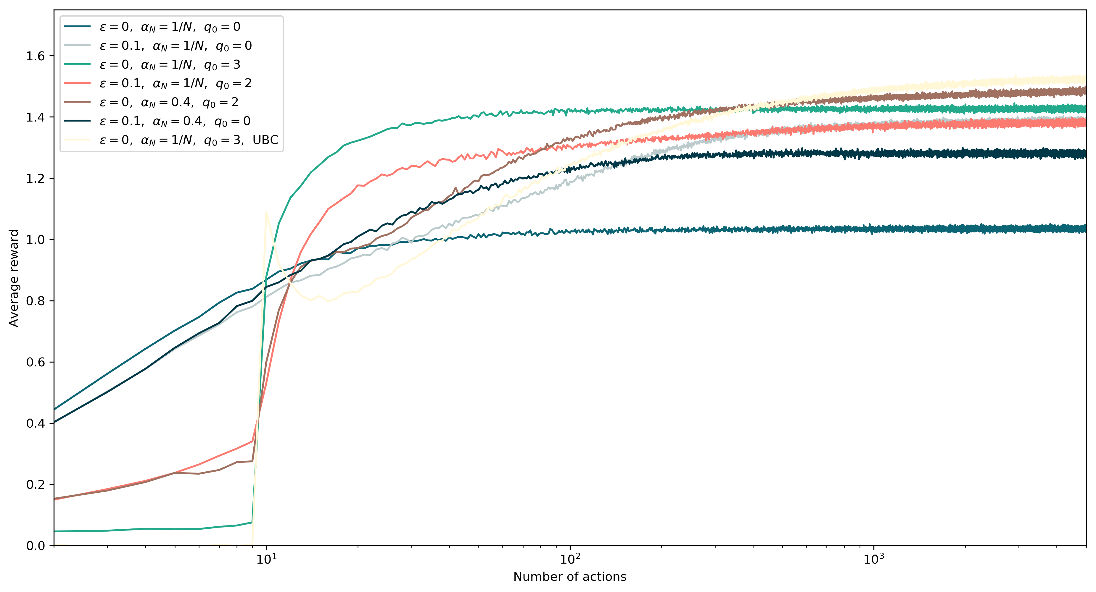
Here’s some algorithm examples. Most of them are epsilon-greedy, some with weight decay of the estimated action value and some use the concept of optimistic initial values. The last shows the upper confidence bound (UCB) algorithm:
n_parallel = 50000
total_steps = 5000
K = 10
fig, ax = plt.subplots(1, figsize=(15, 8))

model = Model(K=K, total_steps=total_steps, n_parallel=n_parallel, epsilon=0, initial_q=0, alpha_n=lambda n:1/n).run_simulation()
ax.plot(model.rewards_t, label='$\\varepsilon=0$,  $\\alpha_N=1/N$,  $q_0=0$')

model = Model(K=K, total_steps=total_steps, n_parallel=n_parallel, epsilon=0.1, initial_q=0, alpha_n=lambda n:1/n).run_simulation()
ax.plot(model.rewards_t, label='$\\varepsilon=0.1$,  $\\alpha_N=1/N$,  $q_0=0$')

model = Model(K=K, total_steps=total_steps, n_parallel=n_parallel, epsilon=0, initial_q=3, alpha_n=lambda n:1/n).run_simulation()
ax.plot(model.rewards_t, label='$\\varepsilon=0$,  $\\alpha_N=1/N$,  $q_0=3$')

model = Model(K=K, total_steps=total_steps, n_parallel=n_parallel, epsilon=0.1, initial_q=2, alpha_n=lambda n:1/n).run_simulation()
ax.plot(model.rewards_t, label='$\\varepsilon=0.1$,  $\\alpha_N=1/N$,  $q_0=2$')

model = Model(K=K, total_steps=total_steps, n_parallel=n_parallel, epsilon=0, initial_q=2, alpha_n=lambda n:0.4).run_simulation()
ax.plot(model.rewards_t, label='$\\varepsilon=0$,  $\\alpha_N=0.4$,  $q_0=2$')

model = Model(K=K, total_steps=total_steps, n_parallel=n_parallel, epsilon=0.1, initial_q=0, alpha_n=lambda n:0.4).run_simulation()
ax.plot(model.rewards_t, label='$\\varepsilon=0.1$,  $\\alpha_N=0.4$,  $q_0=0$')

model = UCB_Model(K=K, total_steps=total_steps, n_parallel=n_parallel, epsilon=0, initial_q=3, alpha_n=lambda n:1/n).run_simulation()
ax.plot(model.rewards_t, label='$\\varepsilon=0$,  $\\alpha_N=1/N$,  $q_0=3$,  UBC')

ax.set(xscale='log', xlim=(2, 5000))
ax.set(xlabel='Number of actions', ylabel='Average reward', ylim=(0,1.75))
ax.legend()