Iterative policy evaluation
The iterative policy evaluation can be used to optimize the decision making in a Markov Decision Process (MDP). In such a problem we have an agent, which can perform actions in an environment. The action brings the agent from a state s to a state s’ and doing so, the agent receives a reward r. The actions available and the reward depend only on the state s the agent is currently in. There is no memory in the system, the state the agent is in contains all the information: the previous state history does not make any difference.
The goal of the agent is to perform actions that maximize the expected reward during a given task. The task can be episodic, i.e. there is an end state like in example a chess game. After the end state is reached the agent state is reset. The task can also be continuous, and it goes on indefinitely. In this latter case, the expected reward must be normalized to avoid divergence, for example by introducing an exponential decay of the rewards while moving into the future.
The maze
Here we use a toy model to show how to optimize the decision-making process of an agent using iterative policy evaluation. Here we will not describe the theory in any detail, which can be found here, but we will just show the code which completes the task.
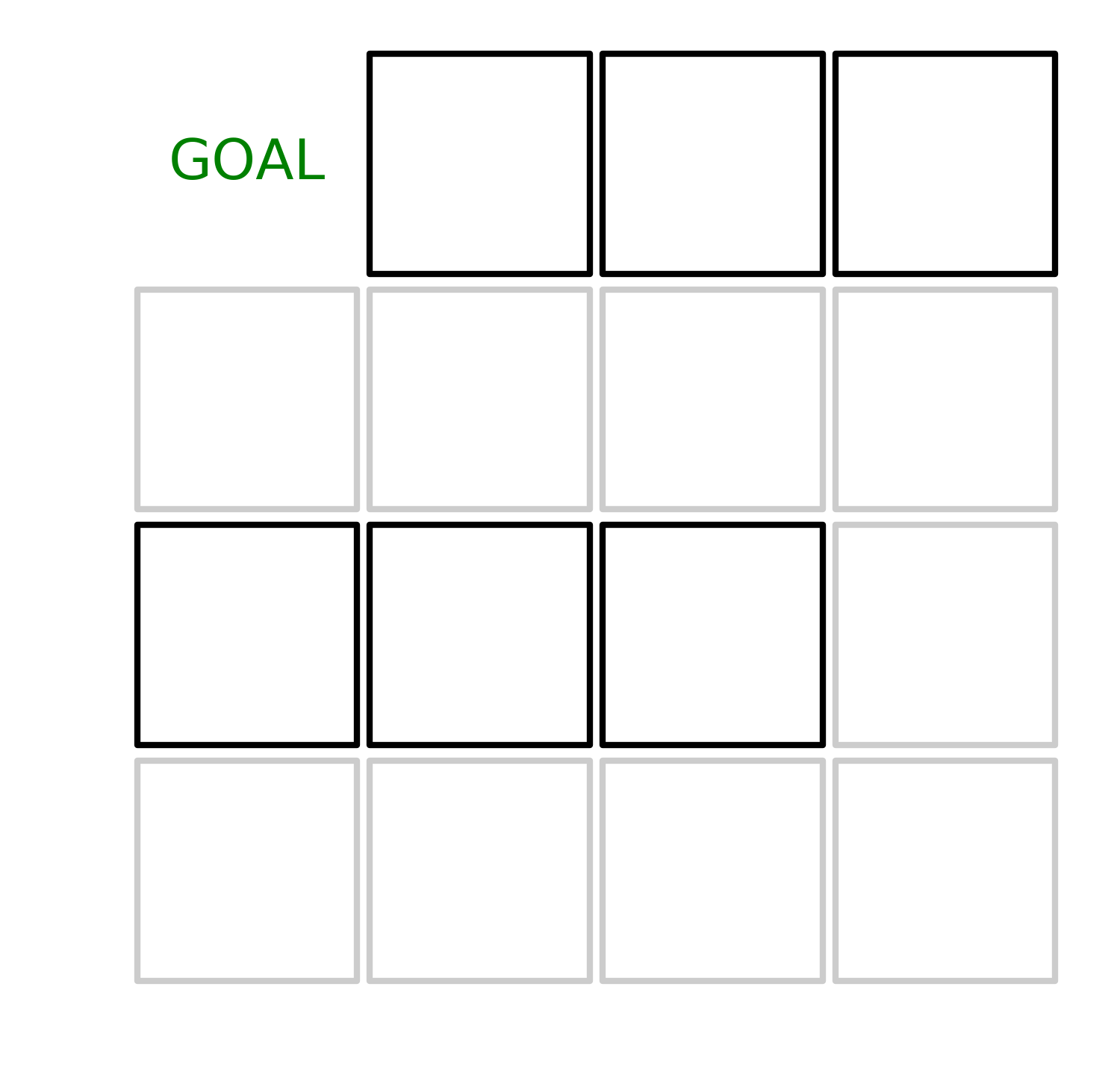
The problem is simple: we have a 4 by 4 grid, the agent can move in any direction and the goal is to reach to top left corner of the grid. Every movement costs to the agent a negative reward of -1 except for some special cells, identified by darker edges, which have a negative reward of -5.
To find the optimal path, the agent needs to follow to reach the target from any given state we use the iterative policy evaluation method. This method consists in alternating value function evaluation and policy improvement. The value function evaluation is obtained by using the Bellman equations, i.e. estimating the expected reward the agent receives to complete the task with a given policy. A policy is a set of rules which defines the action to be taken in a given state. The initial policy is to move randomly in any given direction.
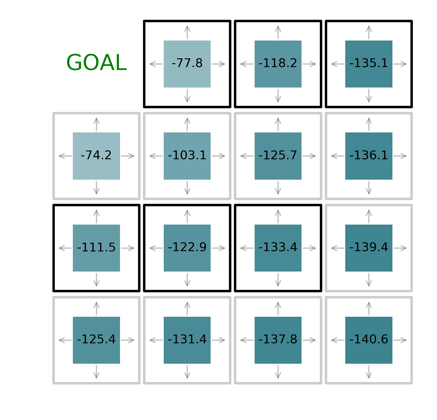
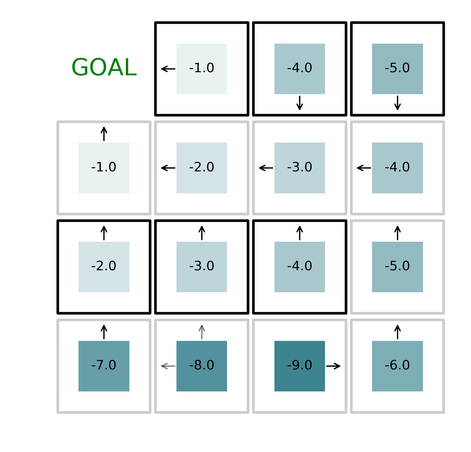
Here we see that it costs around 70 to reach the goal from a nearby state, while it cost around twice the value starting from the opposite corner. The policy improvement consists of defining a new policy that consists of taking the action which brings the agent in the state which corresponds to the maximum reward.

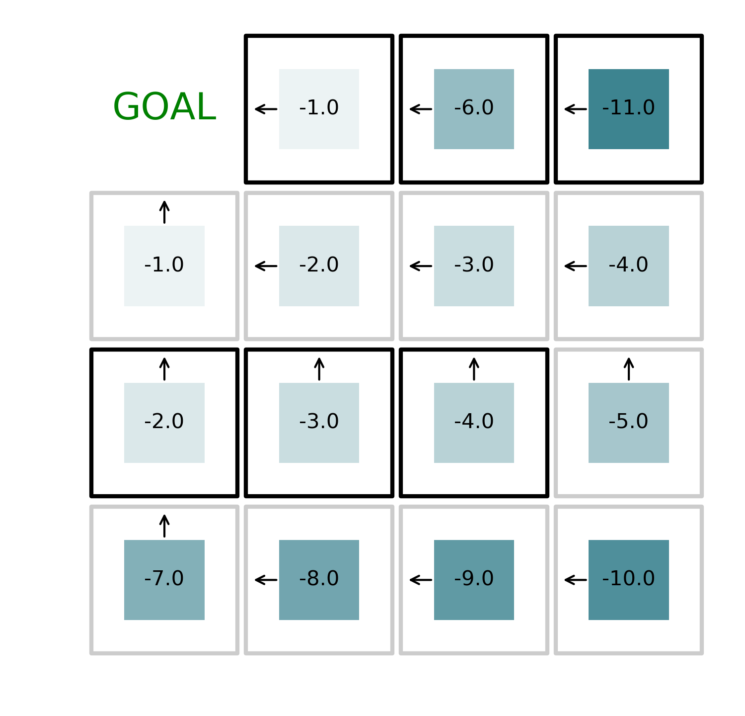
As we can see in the figure above, the new policy for the bottom left state is to move the agent left. This because the “left” state corresponds to a reward of -137.8, which is greater than the “up” state, which has a reward of 139.4.
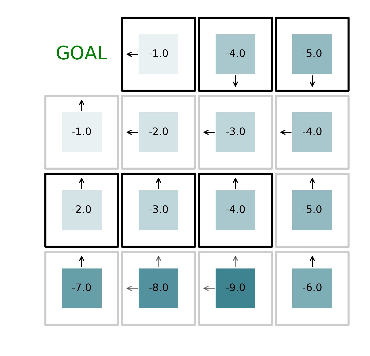
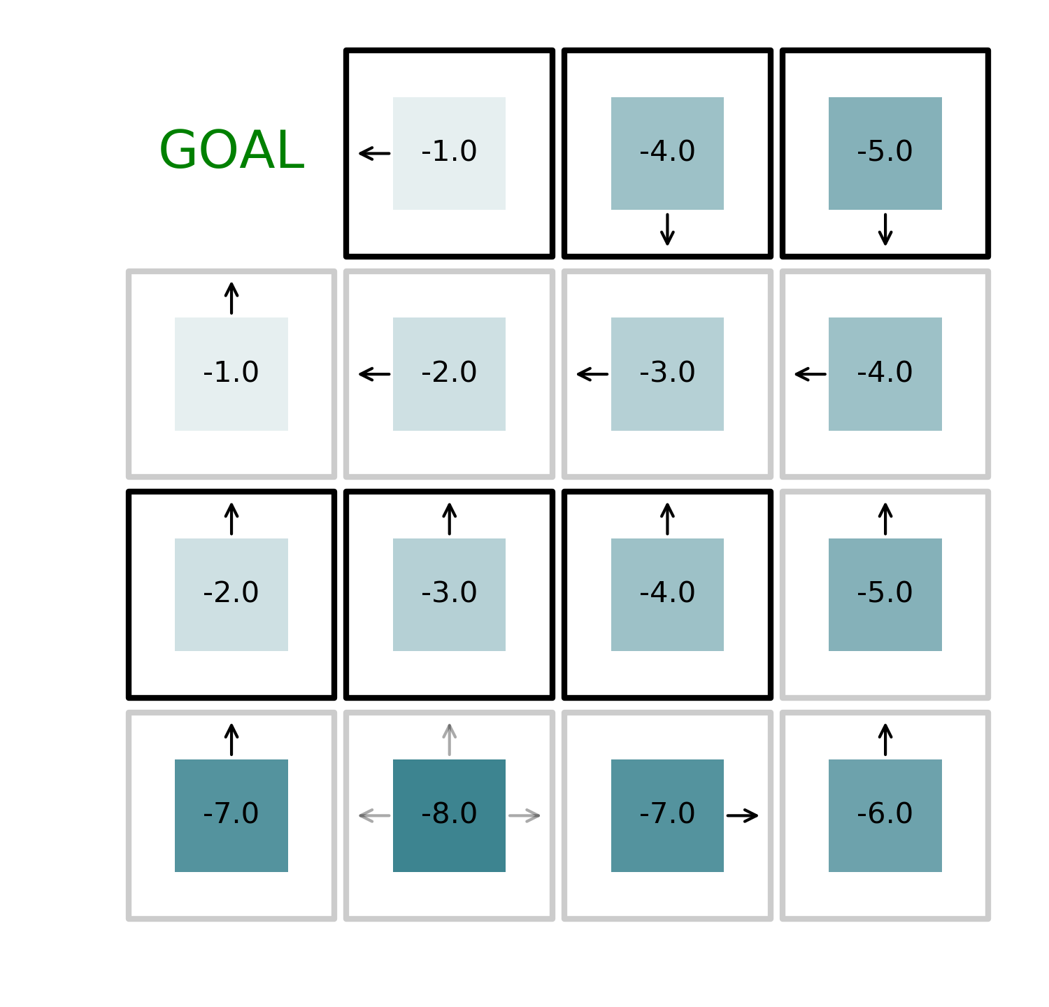
By iteratively alternating value function evaluation and policy improvement, we can find the optimal solution to the problem in just 4 iterations as shown in the figures below.


The code
Here’s the code to reproduce the optimization of the path to reach the end of the maze.
import numpy as np
import matplotlib.pyplot as plt

SIZE = 4

def do_action(x, y, action):
    if action==0:
        return x, min(y+1, SIZE-1)
    if action==1:
        return x, max(y-1, 0)
    if action==2:
        return min(x+1, SIZE-1), y
    if action==3:
        return max(x-1, 0), y

def action_argmax(x, y, v, reward):
    values = []
    for action in range(4):
        xp, yp = do_action(x, y, action)
        values.append(v[xp, yp] + reward[xp, yp])
    return np.where(values==np.max(values))[0]

def define_reward():
    reward = -np.ones([SIZE,SIZE])
    reward[1:, 0] = -5
    reward[:-1, 2] = -5
    return reward

def loop_states():
    for x in range(SIZE):
        for y in range(SIZE):
            if not((x==0 and y==0)):
                yield x, y

def estimate_value_function(v0, v1, reward, pi, delta_max=0.001):
    delta = 1
    while delta > delta_max:
        for x, y in loop_states():
            for action in range(4):
                xp, yp = do_action(x, y, action)
                v1[x, y] = v1[x, y] + pi[x, y, action]*(reward[xp, yp] + v0[xp, yp])
        delta = np.sum(np.abs(v0-v1))
        v0, v1 = v1, np.zeros([SIZE,SIZE])
    return v0, v1

def initialize_policy():
    return np.ones([SIZE,SIZE,4])*0.25

def initialize_state_values():
    return np.zeros([SIZE,SIZE]), np.zeros([SIZE,SIZE])

def plot_value_function(v, reward, pi):
    fig, ax = plt.subplots(1, figsize=(SIZE+1, SIZE+1-0.2))
    ax.set(xlim=(-0.5,SIZE-0.5), ylim=(SIZE-0.5, -0.5))
    for x, y in loop_states():
        ax.text(x, y, f'{v[x, y]:.1f}', ha='center', va='center')
        ax.scatter(x, y, marker='s', s=5000, edgecolors = 'black',color='none',
                   alpha=-(reward[x,y])/np.max(np.abs(reward)), linewidths=2)
        ax.scatter(x, y, marker='s', s=1500, edgecolors = 'none', color='#0c6575',
                   alpha=(-v[x,y])/np.max(np.abs(v))*0.8, linewidths=2)
        ax.annotate("", xy=(x, y+0.45), xytext=(x, y+0.25),
                    arrowprops=dict(arrowstyle="->", alpha=pi[x, y, 0]))
        ax.annotate("", xy=(x, y-0.45), xytext=(x, y-0.25),
                    arrowprops=dict(arrowstyle="->", alpha=pi[x, y, 1]))
        ax.annotate("", xy=(x+0.45, y), xytext=(x+0.25, y),
                    arrowprops=dict(arrowstyle="->", alpha=pi[x, y, 2]))
        ax.annotate("", xy=(x-0.45, y), xytext=(x-0.25, y),
                    arrowprops=dict(arrowstyle="->", alpha=pi[x, y, 3]))
    ax.text(0, 0, 'GOAL', ha='center', va='center', color='green', size=18)
    plt.axis('off')
    plt.tight_layout()
    return fig


def optimize_path():
    reward = define_reward()
    pi = initialize_policy()
    v0, v1 = initialize_state_values()

    while True:
        v0, v1 = estimate_value_function(v0, v1, reward, pi)

        yield plot_value_function(v0, reward, pi)

        for x, y in loop_states():
            pi[x, y, :] = 0
            max_actions = action_argmax(x, y, v0, reward)
            for action in max_actions:
                pi[x, y, action] = 1/max_actions.shape[0]

        yield plot_value_function(v0, reward, pi)
s = optimize_path()
for _ in range(8):
    next(s)