Monte Carlo RL
A Markov decision process (MDP) can be optimized using various reinforcement learning techniques. Sometimes the best way to optimize the decision process is using the Monte Carlo sampling technique, in particular, when:
- The model of the environment is very big, and it is difficult to store it.
- The size of the MDP is big since the computation needed to update the value of each state depends only on the length of the episode and not on the size of the MDP.
- One needs to evaluate each state independently.
Toy model
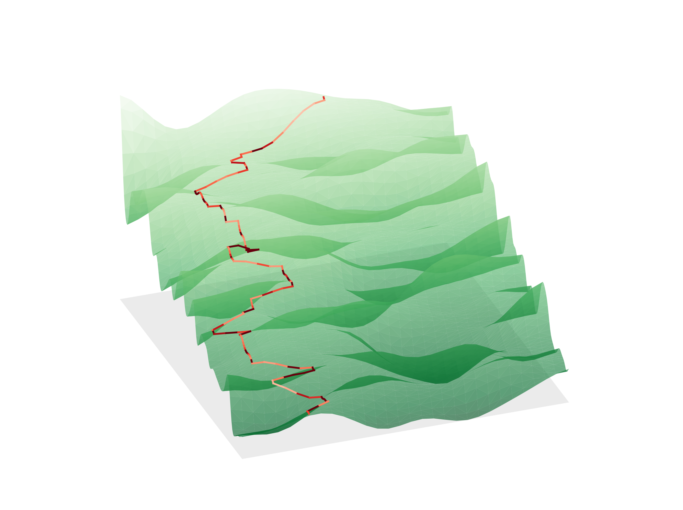
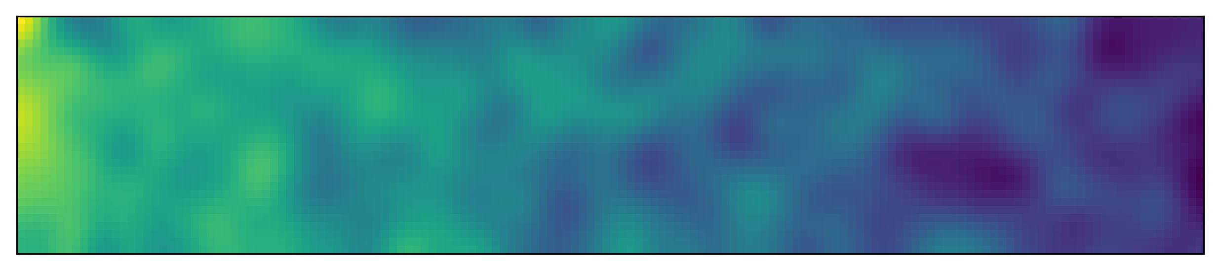
To illustrate how one can use the Monte Carlo technique we use a simple toy model consisting of a track. The agent starts on one side and moves towards the opposite one, choosing the best path to avoid uphill segments. He receives 0 reward when going downhill, a negative reward when turning and a negative reward when riding uphill, proportional to the steepness.
SIZE_X = 30
SIZE_T = 150

def do_action(x, t, action):
    if action==0:
        return x, t+1
    if action==1:
        return min(x+1, SIZE_X-1), t+1
    if action==2:
        return max(x-1, 0), t+1

def calculate_reward(x, t, action):
    u_init = field[x, t]
    xp, tp = do_action(x, t, action)
    u_fin = field[xp, tp]
    movement_reward = 0 if action==0 else -0.05
    return min(u_fin-u_init, 0)
The track is randomly generated as follows:
import numpy as np
import matplotlib.pyplot as plt
from scipy import ndimage

def bin_image(image, binsize_x=1, binsize_y=None, agg_func=np.sum):
    sy, sx = image.shape
    if not binsize_y:
        binsize_y = binsize_x

    y_bins, x_bins = sy // binsize_y, sx // binsize_x
    crop = np.ogrid[(sy % binsize_y)//2: sy-((sy % binsize_y)//2+(sy%binsize_y)%2),
                   (sx % binsize_x)//2: sx-((sx % binsize_x)//2+(sx%binsize_x)%2)]
    cropped = image[tuple(crop)]
    x_agg = agg_func(cropped.reshape(cropped.shape[0], x_bins, binsize_x), axis=2)
    return agg_func(x_agg.reshape(y_bins, binsize_y, x_agg.shape[1]), axis=1)


np.random.seed(0)
field = (np.random.random([300, 1500])-0.5)
field = ndimage.gaussian_filter(field, 25)
field = bin_image(field, binsize_x=10)
field = field - np.ones(field.shape)*np.arange(field.shape[1])*0.02

fig, ax = plt.subplots(1, figsize=(22, 2))
ax.imshow(field)
Helper functions
def initialize_policy():
    return np.ones([SIZE_X, SIZE_T, 3]) * (1/3)

def initialize_state_values():
    return np.zeros([SIZE_X, SIZE_T])

def action_argmax(x, t, v):
    values = []
    for action in range(3):
        xp, tp = do_action(x, t, action)
        values.append(v[xp, tp] + calculate_reward(x, t, action))
    return np.where(values==np.max(values))[0]

def off_policy_action():
    return np.random.randint(3)

def loop_states():
    for t in range(SIZE_T-1):
        for x in range(SIZE_X):
            yield x, t

def plot_path(pi, x0=5):
    fig, ax = plt.subplots(1, figsize=(22, 2))
    ax.imshow(field)

    x = x0
    reward = 0
    for t in range(pi.shape[1]-1):
        ax.scatter(t, x, color='red')
        action = np.random.choice(3, p=pi[x, t, :]/np.sum(pi[x, t, :]))
        reward = reward + calculate_reward(x, t, action)
        x, _ = do_action(x, t, action)
    return fig, reward
Exploring start Monte Carlo
If we perform actions using a completely greedy policy, i.e. always choosing the action that leads to the highest values state, we cannot be sure to explore the whole phase space. One possibe solution is to use exploring starts. The idea is to select the first state and the first action complitly at random. This way we can ensure taht all the phase space will be eventually explored.
def update_action_value_function_MC(Q, Q_n, pi):
    episodes = []
    x = np.random.randint(SIZE_X)
    t = np.random.randint(SIZE_T-1)
    action = np.random.randint(3)
    reward = calculate_reward(x, t, action)
    episodes.append((x, t, action, reward))

    for step in range(SIZE_T-t-3):
        x, t = do_action(x, t, action)
        action = np.argmax(pi[x, t, :])
        reward = calculate_reward(x, t, action)
        episodes.append((x, t, action, reward))

    G = 0
    gamma = 1
    for episode in reversed(episodes):
        x, t, a, r = episode
        G = gamma*G + r
        Q_n[x, t, a] = Q_n[x, t, a] + 1
        Q[x, t, a] = Q[x, t, a] + 1/Q_n[x, t, a] * (G - Q[x, t, a])
    return Q, Q_n

def optimize_path_MC():
    pi = initialize_policy()
    v = initialize_state_values()
    Q = np.zeros([SIZE_X, SIZE_T, 3])
    Q_n = np.zeros([SIZE_X, SIZE_T, 3])

    while True:
        Q, Q_n = update_action_value_function_MC(Q, Q_n, pi)
        for x, t in loop_states():
            pi[x, t, :] = 0
            max_actions = np.where(Q[x, t, :]==np.max(Q[x, t, :]))[0]
            for action in max_actions:
                pi[x, t, action] = 1/max_actions.shape[0]
        yield pi
Epsilon greedy MC
A second strategy to avoid using exploring starts consists in exploiting an epsilon-greedy strategy, which again garantees to explore the full phase space eventually. The problem with epsilon greedy policy is that it is suboptimal both for acting and learning.
def update_action_value_function_MC_eps(Q, Q_n, pi):
    episodes = []
    x = np.random.randint(SIZE_X)
    t = 0
    action = np.random.randint(3)
    reward = calculate_reward(x, t, action)
    episodes.append((x, t, action, reward))

    for step in range(SIZE_T-t-3):
        x, t = do_action(x, t, action)
        if np.random.random() < 0.1:
            action = np.random.randint(3)
        else:
            action = np.argmax(pi[x, t, :])
        reward = calculate_reward(x, t, action)
        episodes.append((x, t, action, reward))

    G = 0
    gamma = 1
    for episode in reversed(episodes):
        x, t, a, r = episode
        G = gamma*G + r
        Q_n[x, t, a] = Q_n[x, t, a] + 1
        Q[x, t, a] = Q[x, t, a] + 1/Q_n[x, t, a] * (G - Q[x, t, a])
    return Q, Q_n

def optimize_path_MC_eps():
    pi = initialize_policy()
    v = initialize_state_values()
    Q = np.zeros([SIZE_X, SIZE_T, 3])
    Q_n = np.zeros([SIZE_X, SIZE_T, 3])

    while True:
        Q, Q_n = update_action_value_function_MC_eps(Q, Q_n, pi)
        for x, t in loop_states():
            pi[x, t, :] = 0
            max_actions = np.where(Q[x, t, :]==np.max(Q[x, t, :]))[0]
            for action in max_actions:
                pi[x, t, action] = 1/max_actions.shape[0]
        yield pi
Off policy learning MC
A third possible strategy is to exploit off-policy learning, which improve and evaluate a different policy from the one used to select actions. Naturally, the behavioural policy (the one choosing the action) must cover the target policy.
def update_action_value_function_MC_offpol(Q, C, pi):
    episodes = []
    x = np.random.randint(SIZE_X)
    t = 0
    action = np.random.randint(3)
    reward = calculate_reward(x, t, action)
    episodes.append((x, t, action, reward))
    b = np.ones([SIZE_X, SIZE_T, 3]) * (1/3)


    for step in range(SIZE_T-t-3):
        x, t = do_action(x, t, action)
        action = np.random.choice(3, p=b[x, t, :] / np.sum(b[x, t, :]))
        action = np.random.randint(3)
        reward = calculate_reward(x, t, action)
        episodes.append((x, t, action, reward))

    G = 0
    W = 1
    gamma = 1
    for episode in reversed(episodes):
        x, t, a, r = episode
        G = gamma*G + r
        C[x, t, a] = C[x, t, a] + W
        Q[x, t, a] = Q[x, t, a] + W/C[x, t, a] * (G - Q[x, t, a])
        W = W /b[x, t, a]
    return Q, C

def optimize_path_MC_offpol():
    pi = initialize_policy()
    v = initialize_state_values()
    Q = np.zeros([SIZE_X, SIZE_T, 3])
    C = np.zeros([SIZE_X, SIZE_T, 3])

    while True:
        Q, C = update_action_value_function_MC_offpol(Q, C, pi)
        for x, t in loop_states():
            pi[x, t, :] = 0
            max_actions = np.where(Q[x, t, :]==np.max(Q[x, t, :]))[0]
            for action in max_actions:
                pi[x, t, action] = 1/max_actions.shape[0]
        yield pi
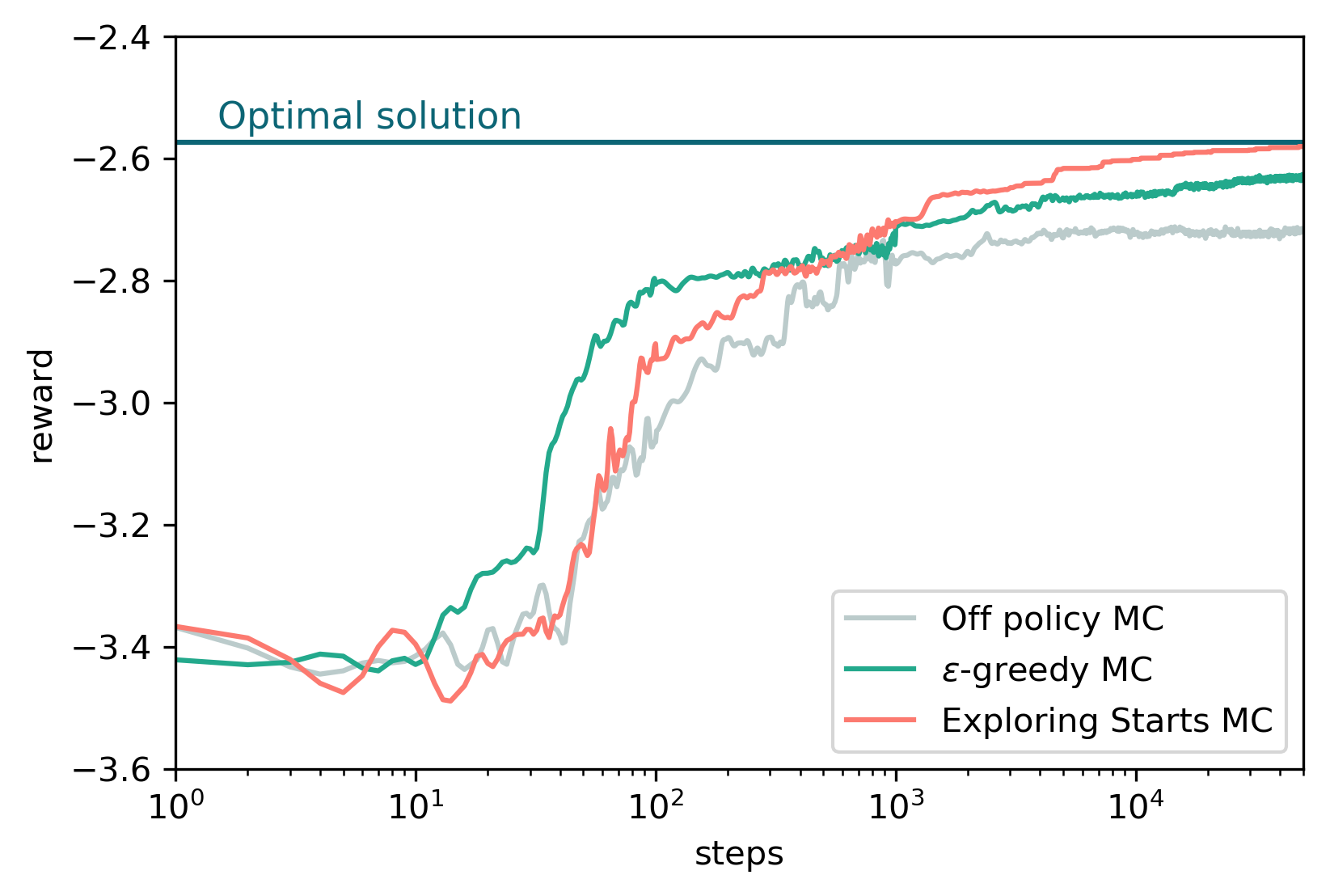
Comparison
Here we show a comparison between of the performances relative to the three algorithm above. We run each simulation as follows in order to average 10 different runs. Each run consists in 50000 steps.
%%time
rewards_list = []
for i in tqdm.tqdm(range(2)):
    s = optimize_path_algorithm() # for example optimize_path_MC_offpol()
    rewards = [get_path_reward(next(s)) for _ in range(10)]
    rewards_list.append(rewards)
The comparison in show in the plot below togheter with the optimal solution obtained using an iterative policy evaluation mathod: