SARSA and Q-learning
Q-learning is a model-free reinforcement learning algorithm that is used to find an optimal policy in a Markov decision process problem. The algorithm learns the action-value function Q=Q(s, a), which describes the value corresponding to a given action, carried out on a given state. Q-learning can work both on-policy and off-policy, and also somewhere in between. A Q-learning variant working on-policy is the SARSA (State Action Reward State Action) algorithm, which, as its name suggests, is based on state-action pairs. Moreover, the expected SARSA algorithm can work both on-policy and off-policy, depending on the choice of the policy. Here we will not describe the algorithms, but we will just use them to solve two different problems (following the Richard S. Sutton and Andrew G. Barto book).
The cliff
In the following we use a simple toy model, called “the cliff” by Richard Sutton and Andrew Barto), to compare Q-learning and SARSA. The task is simple: we have a 12x4 grid, the agent starts from the bottom left corner and its task is to reach the bottom right one. The agent can move in every direction and gets a reward of -1 for each step. If the agent reaches one of the bottom tiles, which is neither the starting nor the ending one, it gets a reward of -100 and it is moved to the starting tile (the bottom left one). The task of the reinforcement learning algorithm finds the best policy to maximize the reward. The chosen policy update is the epsilon-greedy policy.
Here are some libraries and configurations we will use
import matplotlib.pyplot as plt
import numpy as np
import tqdm
from cycler import cycler
from pathlib import Path

colors = ['#0c6575', '#bbcbcb', '#23a98c', '#fc7a70','#a07060',
          '#003847', '#FFF7D6', '#5CA4B5', '#eeeeee']
plt.rcParams['axes.prop_cycle'] = cycler(color = colors)

temp_path = Path('../temp')
The possible actions of the agents are:
def do_action(x, y, action):
    if action==0:
        x, y = x, y+1
    elif action==1:
        x, y = x+1, y
    elif action==2:
        x, y = x, y-1
    elif action==3:
        x, y = x-1, y

    x = np.clip(x, 0, SIZE_X - 1)
    y = np.clip(y, 0, SIZE_Y - 1)

    if (y==0 and x>0 and x<(SIZE_X - 1)):
        x, y = 0, 0
        reward = -100
    elif (y==0 and x==(SIZE_X - 1)):
        reward = 0
    else:
        reward = -1

    return x, y, reward
The epsilon-greedy action selection is given by:
def get_greedy_action(actions):
    best_actions = np.argwhere(actions==np.max(actions)).flatten()
    return np.random.choice(best_actions)

def select_action(x, y, Q, t, epsilon=0.1):
    if np.random.random() < epsilon:
        return np.random.randint(4)
    else:
        return get_greedy_action(Q[y, x, :])
A single step and optimization is showed below. Q is the action-value function, t is the time step, alg can be set as sarsa or as q to select between q-learning and SARSA algorithms. alpha is the learning rate and gamma is the discount factor.
def run_one_episode(Q, t, return_steps=False, alg='sarsa', alpha=0.5, gamma=1):
    x, y = 0, 0
    if return_steps:
        xs, ys = [0], [0]
    action = select_action(x, y, Q, t)
    sum_rewards = 0
    while True:
        x_next, y_next, reward = do_action(x, y, action)
        if return_steps:
            xs.append(x_next)
            ys.append(y_next)
        sum_rewards = sum_rewards + reward

        action_next = select_action(x_next, y_next, Q, t)
        if alg == 'sarsa':
            Q[y, x, action] = (Q[y, x, action] + alpha*(reward +
                    gamma*Q[y_next, x_next, action_next] - Q[y, x, action]))
        elif alg == 'q':
            Q[y, x, action] = (Q[y, x, action] + alpha*(reward +
                    gamma*np.max(Q[y_next, x_next, :]) - Q[y, x, action]))

        x, y = x_next, y_next
        action = action_next

        # target reached
        if not reward:
            if return_steps:
                return Q, sum_rewards, xs, ys
            else:
                return Q, sum_rewards
The simulation
Here are some utility functions, used to loop between the sates and to plot the average path taken by the two agents.
STEPS = 100
PARALLEL_SIMULATIONS = 150
NUMBER_OF_ACTIONS = 4
S_MARKER = 1500
SIZE_X = 12
SIZE_Y = 4

Q_q = np.zeros([SIZE_Y, SIZE_X, NUMBER_OF_ACTIONS, PARALLEL_SIMULATIONS])
Q_s = np.zeros([SIZE_Y, SIZE_X, NUMBER_OF_ACTIONS, PARALLEL_SIMULATIONS])
rewards_q = np.zeros([STEPS, PARALLEL_SIMULATIONS])
rewards_s = np.zeros([STEPS, PARALLEL_SIMULATIONS])

def loop_states():
    for x in range(Q_q.shape[1]):
        for y in range(Q_q.shape[0]):
            yield x, y

def plot_density_path(ax, xs, ys, color):
    density_path = np.zeros([Q_q.shape[1], Q_q.shape[0]])

    for x, y in zip(xs, ys):
        density_path[x, y] = density_path[x, y] + 1
    density_path = density_path/np.max(density_path)
    for x, y in loop_states():
        ax.scatter(x, y, marker='s', c=color, s=MARKER_SIZE,
                   alpha=density_path[x, y], zorder=10)

def plot_background(axs):
    for ax in axs:
        for x, y in loop_states():
            ax.scatter(x, y, marker='s', s=S_MARKER, color=colors[8])
        [ax.scatter(1+x, 0, marker='s', s=S_MARKER, color='black') for x in range(10)]
        ax.axis('off')
        ax.set(aspect=1)
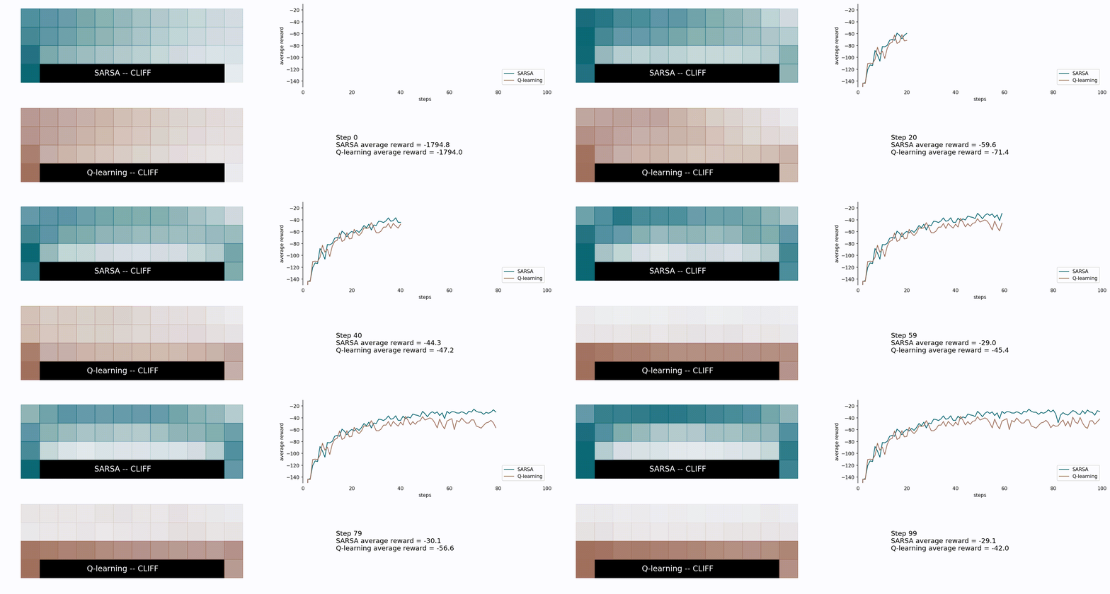
Here’s the comparison between the SARSA (blue) and the Q-learning algorithm (brown).
for step in range(STEPS):
    xs_s, ys_s, xs_q, ys_q = [], [], [], []

    fig, ((ax0, ax1), (ax2, ax3)) = plt.subplots(2, 2, figsize=(20, 7))

    # background
    plot_background(axs=(ax0, ax2))

    # sarsa
    for sim_index in range(PARALLEL_SIMULATIONS):
        Q_s[...,sim_index], sum_rewards_s, xs, ys = run_one_episode(
            Q_s[...,sim_index], step+1, alpha=0.5, alg='sarsa', return_steps=True)
        xs_s, ys_s = xs_s + xs, ys_s + ys
        rewards_s[step, sim_index] = sum_rewards_s
    plot_density_path(ax0, xs_s, ys_s, colors[0])
    ax0.text(5, 0, 'SARSA -- CLIFF', color='white',
             va='center', ha='center', size=16, zorder=20)

    # q-learning
    for sim_index in range(PARALLEL_SIMULATIONS):
        Q_q[...,sim_index], sum_rewards_q, xs, ys = run_one_episode(
            Q_q[...,sim_index], step+1, alpha=0.5, alg='q', return_steps=True)
        xs_q, ys_q = xs_q + xs, ys_q + ys
        rewards_q[step, sim_index] = sum_rewards_q
    plot_density_path(ax2, xs_q, ys_q, colors[4])
    ax2.text(5, 0, 'Q-learning -- CLIFF', color='white',
             va='center', ha='center', size=16, zorder=20)

    x = range(step+1)
    ax1.plot(x, np.mean(rewards_s,1)[:step+1], color=colors[0], label='SARSA')
    ax1.plot(x, np.mean(rewards_q,1)[:step+1], color=colors[4], label='Q-learning')
    ax1.legend(loc=4)
    ax1.set(ylim=(-150, -10), xlim=(0,STEPS), xlabel='steps', ylabel='average reward')
    [ax1.spines[pos].set_visible(False) for pos in ('top', 'right', 'bottom')]
    [tl.set_color('none') for tl in ax1.get_xticklines()];

    ax3.axis('off')
    text_description = f'''
    Step {step}
    SARSA average reward = {np.mean(rewards_s,1)[step]:.1f}
    Q-learning average reward = {np.mean(rewards_q,1)[step]:.1f}
    '''
    ax3.text(0.1, 0.5, text_description, size=14, ha='left', va='center')
    ax3.set(xlim=(0,1), ylim=(0,1))

    fig.savefig(temp_path/f'seq_{step:03d}.jpg', bbox_inches='tight', dpi=150)
    plt.close()

Here we see how the Q-learning algorithm is more greedy but less effective in the long run for this particular problem. It chooses the shorter path, which seems reasonable, but also riskier: given the probability of 10% of a random movement it is possible to fall into the cliff and lose -100 rewards plus the part of the path which was already completed. With that in mind, we can see how the SARSA algorithm is more conservative choosing the longer path, farther from the cliff.