Dectection of pneumothorax using x-ray images
Problem definition
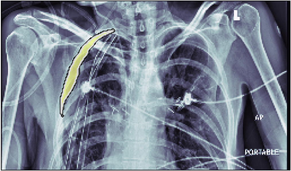
In this post, we will approach the problem of image segmentation using the pneumothorax dataset from kaggle. The problem is straightforward: given an x-ray image of the patient’s chest, you need to detect the presence of pneumothorax issue and spatially locate the region of interest within the image. You are provided with around 100000 x-ray images for training. Each of them comes with a spatial mask locating the pneumothorax problem in the image (if the lung is healthy the mask is just empty). An example of an x-ray image is shown above: the right lung has complications in the top external region.
Neural network model
We choose to approach this problem using a convolutional neural network (the good old friend of image analysis). Instead of training a network from scratch we decided to exploit the VGG-16 network model, pre-trained on the imagenet dataset. The idea is to exploit the first layers of this network, which are already trained to “understand” the very low-level features of an image, such as edges and extremely simple patterns. Since the imagenet dataset contains more than 14 million images, we want to exploit the ability of the trained VGG-16 network to extract the most important low lever features from an image and transfer this “knowledge” to our problem.
Since we are interested in finding the position of the possible lung problem, it makes sense not to exit from the convolutional network structure using dense layers. Instead, one can use a U-type network, similar to the one used in autoencoders: in the first section of the network, we extract the most important features by applying convolutional layers and max-pooling to reduce the size of the image representation and increase the number of channels. In the second half, instead, we use a combination of up-sampling and convolutional layers to reduce the number of channels to just one and increase the image representation size back to the original one.
Importing the images
First of all, we need to import the training dataset and split it into train/dev/test sets. Here we create two lists containing the file paths of the training images together with the respective mask. Moreover, we shuffle these lists and we split them in train/dev/test with a proportion of 250/40/40.
import glob
import random
random.seed(2)

xray_path = f'{root_path}data/train/*'
mask_path = f'{root_path}data/masks/*'
xray_files = sorted(glob.glob(xray_path))
mask_files = sorted(glob.glob(mask_path))

c = list(zip(xray_files, mask_files))
random.shuffle(c)
xray_files, mask_files = zip(*c)

batch_size = 32

train_len = 250 * batch_size
dev_len = 40 * batch_size
test_len = 40 * batch_size

X_train_files = xray_files[:train_len]
y_train_files = mask_files[:train_len]

X_dev_files = xray_files[train_len:train_len+dev_len]
y_dev_files = mask_files[train_len:train_len+dev_len]

X_test_files = xray_files[train_len+dev_len:train_len+dev_len+test_len]
y_test_files = mask_files[train_len+dev_len:train_len+dev_len+test_len]
Then, we want to make sure that the train/dev/test contains images with zero masks (without any detectable lung problem) in the same proportion.
from keras.preprocessing.image import load_img
from keras.preprocessing.image import img_to_array

with_mask = []
for i, f in enumerate(y_train_files):
    m = np.sum(img_to_array(load_img(f, color_mode='grayscale')))
    with_mask.append(m>1)
train_positive = np.mean(with_mask)

with_mask = []
for i, f in enumerate(y_dev_files):
    m = np.sum(img_to_array(load_img(f, color_mode='grayscale')))
    with_mask.append(m>1)
dev_positive = np.mean(with_mask)

with_mask = []
for i, f in enumerate(y_test_files):
    m = np.sum(img_to_array(load_img(f, color_mode='grayscale')))
    with_mask.append(m>1)
test_positive = np.mean(with_mask)

print('Images with mask:')
print(f'Train:{train_positive}, dev:{dev_positive}, test:{test_positive}')
Images with mask:
Train:0.22075, dev:0.22734375, test:0.2296875
As we can see the split is good: train, dev and test sets contain about the same percentage of images with lung issues (around 22-23%).
Using Google colab
Since at the moment we have no access to a local GPU, which is essential to train a conv net, we exploit Google colab free Jupiter notebook. We found out the major limitation of this approach is the low speed in loading the images from the hard drive to the memory, resulting in a very severe performance issue. When using Colab one can store the training files on a google drive folder and load them directly from there. The problem rise as soon as one try to load more then a couple of hundreds of images: at first the process is quite fast and requires for 5 to 10 ms for each image, which is ok, but, after a while, the speed drastically drop (apparently for no reason) and the loading time becomes of the order of half of a second, an extremely huge bottleneck in the pipeline which practically results in the freezing of the training computation. Since the dataset is quite small in size (of the order of Gb), we decided to load it all in memory. We used the HDF5 data format to store all the dataset, and load just this one big file on our google drive folder.
import h5py

data_filename = f'{root_path}data/data.h5'
with h5py.File(data_filename, "w") as out:

    data_type = 'uint8'

    out.create_dataset("X_train",(len(X_train_files),256,256,1),dtype=data_type)
    out.create_dataset("Y_train",(len(X_train_files),256,256,1),dtype=data_type)
    out.create_dataset("X_dev",(len(X_dev_files),256,256,1),dtype=data_type)
    out.create_dataset("Y_dev",(len(X_dev_files),256,256,1),dtype=data_type)
    out.create_dataset("X_test",(len(X_test_files),256,256,1),dtype=data_type)
    out.create_dataset("Y_test",(len(X_test_files),256,256,1),dtype=data_type)

    for index in range(len(y_train_files)):
        out['X_train'][index, :, :, :] = img_to_array(load_img(
            X_train_files[index], color_mode='grayscale')).astype(data_type)
        out['Y_train'][index, :, :, :] = img_to_array(load_img(
            y_train_files[index], color_mode='grayscale')).astype(data_type)

    for index in range(len(y_dev_files)):
        out['X_dev'][index, :, :, :] = img_to_array(load_img(
            X_dev_files[index], color_mode='grayscale')).astype(data_type)
        out['Y_dev'][index, :, :, :] = img_to_array(load_img(
            y_dev_files[index], color_mode='grayscale')).astype(data_type)

    for index in range(len(y_test_files)):
        out['X_test'][index, :, :, :] = img_to_array(load_img(
            X_test_files[index], color_mode='grayscale')).astype(data_type)
        out['Y_test'][index, :, :, :] = img_to_array(load_img(
            y_test_files[index], color_mode='grayscale')).astype(data_type)
Data augmentation
To avoid overfitting we decide to use a data augmentation technique widely used during the training of neural networks for computer vision tasks. The idea is never to train the network with the same image twice: every time the image is presented to the network to perform one gradient descent step, it is randomly modified by a given transformation chosen at random within a given set. To do this, we exploit the ImageDataGenerator Keras builtin function:
from keras.preprocessing.image import ImageDataGenerator

image_randomiser = ImageDataGenerator(
    rotation_range=10,
    width_shift_range=0.02,
    height_shift_range=0.02,
    zoom_range=0.02,
    fill_mode='nearest',
    horizontal_flip=True)
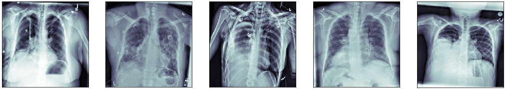
Here’s an example of 5 generated training images. One can see that each one has a different zoom, rotation angle, and stretch. All these modifications are not relevant for the problem of identifying the ill region of the lung, therefore, they act as data regularizers, preventing the model to learn spurious features.
Building up generators
To never feed the network with the same image twice we can take advantage of python generators. The Keras library has a special fit function, fit_generator, which does take as input a generator of X and y data, instead of the data itself. This allows for very convenient solutions, such as on the fly random transformation or loading the data as a stream (very useful for huge datasets which do not fit into the memory).
In our case, since the data is small enough, we decided to load everything in memory. The task of the generator is to randomly transform the images and to finally yield them as batches of size 32. As we can see, the create_data_random_generator exploit the Keras ImageDataGenerator to generate a random transformation to apply both at the lung image and to the corresponding mask. Notice we also create the simple create_data_generator generator, which has no transformation in it. This will be used to manage the data of the dev and test set.
def create_data_generator(X, y, batch_size):
    number_of_samples = X.shape[0]
    print(f'Creating generator from {number_of_samples} samples')

    index = 0
    while True:
        data_X = np.zeros([batch_size, 256, 256, 1])
        data_y = np.zeros([batch_size, 256, 256, 1])

        for i in range(batch_size):
            data_X[i, ...] = X[index % number_of_samples,...]/255.
            data_y[i, ...] = y[index % number_of_samples,...]/255.
            index = index + 1

        data_X = data_X * np.ones([batch_size, 256, 256, 3])
        yield data_X, data_y


def create_data_random_generator(X, y, batch_size):

    image_randomiser = ImageDataGenerator(
        rotation_range=10,
        width_shift_range=0.02,
        height_shift_range=0.02,
        zoom_range=0.02,
        fill_mode='nearest',
        horizontal_flip=True)


    number_of_samples = X.shape[0]
    print(f'Creating generator from {number_of_samples} samples')

    index = 0
    while True:
        data_X = np.zeros([batch_size, 256, 256, 1])
        data_y = np.zeros([batch_size, 256, 256, 1])

        transformation = image_randomiser.get_random_transform(img_shape=(256,256,1))

        for i in range(batch_size):
            data_X[i, ...] = image_randomiser.apply_transform(
                        X[index % number_of_samples,...]/255., transformation)

            data_y[i, ...] = image_randomiser.apply_transform(
                        y[index % number_of_samples,...]/255., transformation)
            index = index + 1

        data_X = data_X * np.ones([batch_size, 256, 256, 3])
        yield data_X, data_y
Finally, we can create the generators for the train, the dev, and the test set, by loading the dataset form the HDF5 file:
with h5py.File(data_filename, 'r') as f:
    train_generator = create_data_random_generator(
        f['X_train'][()], f['Y_train'][()], 32)
    dev_generator = create_data_generator(f['X_dev'][()], f['Y_dev'][()], 32)
    test_generator = create_data_generator(f['X_test'][()], f['Y_test'][()], 32)
Neural network conv model
For the first part of our model, we choose to exploit the VGG-16 pre-trained model, which is available directly from the Keras library. As we can see, together with the model, we load the weights resulting from the training of VGG-16 net on the imagenet dataset.
from keras.applications import VGG16

conv_base = VGG16(weights = 'imagenet',
                  include_top = False,
                  input_shape = (256, 256, 3))
Since we are interested in extracting just the lower features from the images, and not something related to real object identification, we exclude the final set of three convolutional layers. Finally, we set this model not to be trainable for the first stage of gradient descent.
conv_base_crop= Model(inputs=conv_base.layers[0].input,
                      outputs=conv_base.layers[-5].output)
conv_base_crop.trainable=False
conv_base_crop.summary()
_________________________________________________________________
Layer (type)                 Output Shape              Param #
=================================================================
input_1 (InputLayer)         (None, 256, 256, 3)       0
_________________________________________________________________
block1_conv1 (Conv2D)        (None, 256, 256, 64)      1792
_________________________________________________________________
block1_conv2 (Conv2D)        (None, 256, 256, 64)      36928
_________________________________________________________________
block1_pool (MaxPooling2D)   (None, 128, 128, 64)      0
_________________________________________________________________
block2_conv1 (Conv2D)        (None, 128, 128, 128)     73856
_________________________________________________________________
block2_conv2 (Conv2D)        (None, 128, 128, 128)     147584
_________________________________________________________________
block2_pool (MaxPooling2D)   (None, 64, 64, 128)       0
_________________________________________________________________
block3_conv1 (Conv2D)        (None, 64, 64, 256)       295168
_________________________________________________________________
block3_conv2 (Conv2D)        (None, 64, 64, 256)       590080
_________________________________________________________________
block3_conv3 (Conv2D)        (None, 64, 64, 256)       590080
_________________________________________________________________
block3_pool (MaxPooling2D)   (None, 32, 32, 256)       0
_________________________________________________________________
block4_conv1 (Conv2D)        (None, 32, 32, 512)       1180160
_________________________________________________________________
block4_conv2 (Conv2D)        (None, 32, 32, 512)       2359808
_________________________________________________________________
block4_conv3 (Conv2D)        (None, 32, 32, 512)       2359808
_________________________________________________________________
block4_pool (MaxPooling2D)   (None, 16, 16, 512)       0
=================================================================
Total params: 7,635,264
Trainable params: 0
Non-trainable params: 7,635,264
_________________________________________________________________
We final part of our model is a sequence of Conv2D layers, to reduce the number of filters, and UpSampling2D layers, to increase the size of the image representation:
from keras import models

doctor_model = models.Sequential()
doctor_model.add(conv_base)

doctor_model.add(Conv2D(64, (3, 3), activation='relu', padding='same'))
doctor_model.add(UpSampling2D((2,2)))
doctor_model.add(Conv2D(32, (3, 3), activation='relu', padding='same'))
doctor_model.add(UpSampling2D((2,2)))
doctor_model.add(Conv2D(32, (3, 3), activation='relu', padding='same'))
doctor_model.add(UpSampling2D((2,2)))
doctor_model.add(Conv2D(16, (3, 3), activation='relu', padding='same'))
doctor_model.add(UpSampling2D((2,2)))
doctor_model.add(Conv2D(8, (3, 3), activation='relu', padding='same'))
doctor_model.add(UpSampling2D((2,2)))
doctor_model.add(Conv2D(1, (3, 3), activation='sigmoid', padding='same'))

doctor_model.summary()
_________________________________________________________________
Layer (type)                 Output Shape              Param #
=================================================================
model_1 (Model)              (None, 16, 16, 512)       7635264
_________________________________________________________________
conv2d_1 (Conv2D)            (None, 16, 16, 32)        147488
_________________________________________________________________
up_sampling2d_1 (UpSampling2 (None, 32, 32, 32)        0
_________________________________________________________________
conv2d_2 (Conv2D)            (None, 32, 32, 16)        4624
_________________________________________________________________
up_sampling2d_2 (UpSampling2 (None, 64, 64, 16)        0
_________________________________________________________________
conv2d_3 (Conv2D)            (None, 64, 64, 16)        2320
_________________________________________________________________
up_sampling2d_3 (UpSampling2 (None, 128, 128, 16)      0
_________________________________________________________________
conv2d_4 (Conv2D)            (None, 128, 128, 8)       1160
_________________________________________________________________
up_sampling2d_4 (UpSampling2 (None, 256, 256, 8)       0
_________________________________________________________________
conv2d_5 (Conv2D)            (None, 256, 256, 1)       73
=================================================================
Total params: 7,790,929
Trainable params: 155,665
Non-trainable params: 7,635,264
_________________________________________________________________
Fit
We fit the model using the binary_crossentropy loss function and Adam as optimizer. We finally save the model as an HDF5 file.
doctor_model.compile(loss='binary_crossentropy',
                    optimizer=optimizers.Adam(lr=2e-5))

out = doctor_model.fit_generator(train_generator,
                                 steps_per_epoch = 250,
                                 epochs=90,
                                 validation_data = dev_generator,
                                 validation_steps = 40,
                                 verbose=1)

doctor_model.save(f'./doctor_model.h5')
Final results
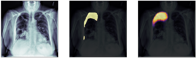
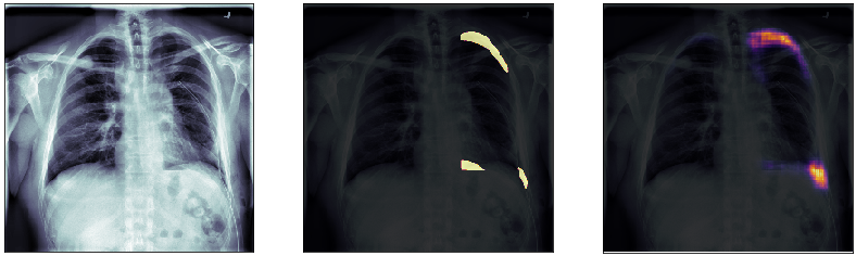
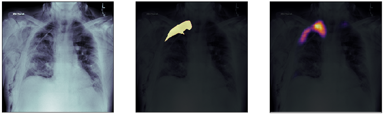
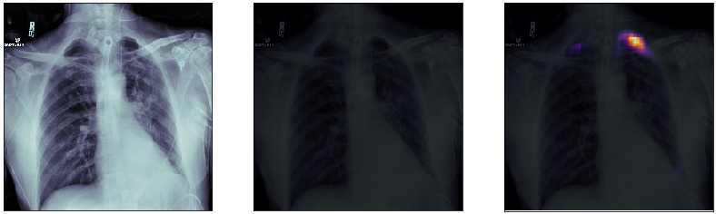
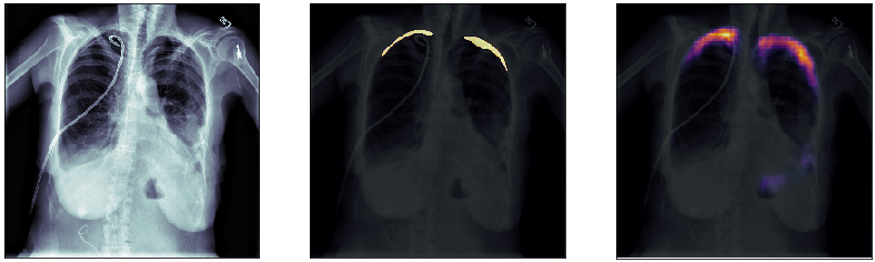
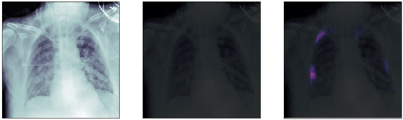
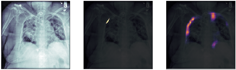
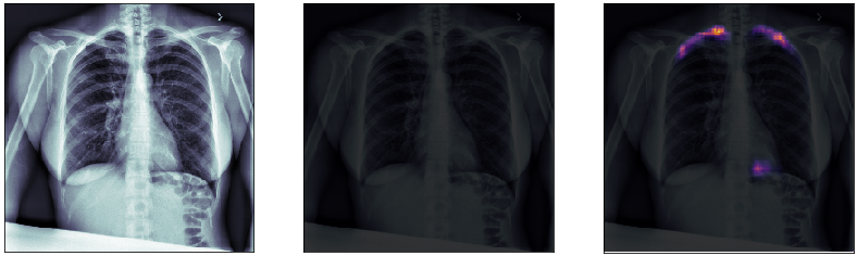
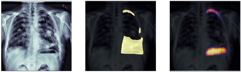
Finally, we plot some model predictions on the test set (data never seen by the network before). On the left, we plot the input image, the x-ray of the lungs. In the middle, we plot the target mask, as indicated by a specialized doctor. On the right, we plot the prediction of our model.
This simple model performs quite well! We also notice that, without having explicitly programmed it to behave like this, most of the errors are false positives and not false negatives, which is great: in this context, it is much better to over-estimate a problem, rather than missing it.