Feature selection
Summary
## Fit + transform available
from sklearn.decomposition import PCA
from sklearn.decomposition import FactorAnalysis
from sklearn.random_projection import GaussianRandomProjection
from sklearn.manifold import Isomap
from sklearn.manifold import LocallyLinearEmbedding
from sklearn.decomposition import TruncatedSVD
from sklearn.decomposition import FastICA

## Only fit_transform
from sklearn.manifold import MDS
from sklearn.manifold import SpectralEmbedding
from sklearn.manifold import TSNE

## Both X and y must be provided
from sklearn.discriminant_analysis import LinearDiscriminantAnalysis

## n_clusters instead of n_components
from sklearn.cluster import FeatureAgglomeration
in the following we plot some examples of dimensionality reduction to plot three different datasets in two dimensions. Moreover, we score the goodness of each algorithm for the given dataset using a simple SVM classifier with cross validation:
from sklearn.model_selection import cross_val_score
from sklearn.svm import SVC
def get_score(X_2D, y):
    clf = SVC(gamma=2, C=1)
    scores = cross_val_score(clf, X_2D, y, cv=5)
    return f'{scores.mean():.2f} (+/- {scores.std()*2:.2f})'
Iris dataset (sklearn)


Wine dataset (sklearn)


Digits dataset (sklearn)


Principal Component Analysis (PCA) for dummies
Project all the points along one direction and measure the variance of the projections position. The direction of the first component is chosen by maximizing this variance. The same idea is followed to choose the remaining components, with the constraint to be orthogonal to the previous ones. Mathematically it can be done by solving the eigenvalues problem using the Singular Value Decomposition and selecting as the most important directions the eigenvectors corresponding to the largest eigenvalues:
from sklearn import datasets
data = datasets.load_iris()
y = data.target
X = data.data
# X = (U @ np.diag(S) @ V)
# S are the eigenvalues in descending order
U, S, V = np.linalg.svd(X, full_matrices=False)

n_components = 2
U = U[:, :n_components]
U = U * S[:n_components]
from sklearn.decomposition import PCA
pca = PCA(n_components=2)
X_2D = pca.fit_transform(X)
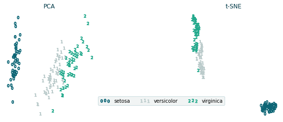
PCA and T-SNE plots
from sklearn.datasets import load_iris
from sklearn.decomposition import PCA
from sklearn.manifold import TSNE
import matplotlib.pyplot as plt
import numpy as np

from cycler import cycler
colors = ['#0c6575', '#bbcbcb', '#23a98c', '#fc7a70','#a07060',
          '#003847', '#FFF7D6', '#5CA4B5', '#eeeeee']
plt.rcParams['axes.prop_cycle'] = cycler(color = colors)


iris_dataset = load_iris()
X = iris_dataset.data
y = iris_dataset.target
y_names = {0:'setosa', 1:'versicolor', 2:'virginica'} # optional, None is fine


X_TSNE = TSNE(n_components=2, random_state=1).fit_transform(X)
X_PCA = PCA(n_components=2).fit_transform(X)


fig, (ax_pca, ax_tsne) = plt.subplots(1, 2, figsize=(10, 4))

for y_class in np.unique(y):
    marker = f'${y_class}$'
    class_mask = (y == y_class)

    ax_tsne.scatter(X_TSNE[class_mask, 0], X_TSNE[class_mask, 1],
              marker=marker, color=colors[y_class],
              label=y_names[y_class] if y_names else f'${y_class}$')
    ax_pca.scatter(X_PCA[class_mask, 0], X_PCA[class_mask, 1],
              marker=marker, color=colors[y_class])

ax_pca.set_title('PCA', color=colors[5])
ax_tsne.set_title('t-SNE', color=colors[5])

ax_tsne.legend(loc='lower left', bbox_to_anchor=(-1, 0.1), ncol=3,
    scatterpoints=3, frameon=True, fancybox=True, framealpha=0.2,
    facecolor=colors[1], edgecolor=colors[0])

ax_pca.axis('off')
ax_tsne.axis('off')
plt.subplots_adjust(left=None, bottom=None, right=None, top=None,
    wspace=1, hspace=None)