Variational Auto Encoder
Variational autoencoders (VAE) are generative models that address the problem of approximate density estimation. Their structure is very similar to standard autoencoders but with the addition of a noisy component at the level of the feature layer. This stochasticity helps to improve the robustness of the model so that every point sampled from the latent space is decoded to a valid output. Randomly sampling from a continuous distribution forces the latent space to encode meaningful representations everywhere, i.e. to be continuously meaningful. In the present example, we employ a normal distribution to generate random noise, which is therefore defined by just two parameters: mean and variance. This code is inspired by Keras’s father François Chollet.
Import modules
import matplotlib.pyplot as plt
import numpy as np
import tensorflow as tf
from tensorflow.keras import Input
from tensorflow.keras.backend import flatten
from tensorflow.keras.layers import Conv2D, Flatten, Dense, Reshape, Conv2DTranspose, Layer, Lambda
from tensorflow.keras.metrics import binary_crossentropy
from tensorflow.keras.models import Model
Model definition
The VAE is basically divided into 3 parts: the encoder, the sampler, and the decoder. The first and the latter have the same structure as a traditional autoencoder, while the sampler layer is responsible for the injection of random noise at the latent space level.
latent_dim = 4
shape_after_encoder = (14, 14, 64)

## encoder model
input_encoder = Input(shape=(28,28,1), name='input_encoder')
x = Conv2D(32, 3, padding='same', activation='relu', name='conv_0')(input_encoder)
x = Conv2D(64, 3, padding='same', activation='relu', strides=(2, 2), name='conv_1')(x)
x = Conv2D(64, 3, padding='same', activation='relu', name='conv_2')(x)
x = Conv2D(64, 3, padding='same', activation='relu', name='conv_3')(x)
x = Flatten(name='flatten_0')(x)
x = Dense(32, activation='relu', name='dense_0')(x)
z_mean = Dense(latent_dim, name='dense_z_mean')(x)
z_log_var = Dense(latent_dim, name='dense_z_log_var')(x)
encoder_model = Model(input_encoder, [z_mean, z_log_var], name='encoder_model')

## sampling layer
def sampling(args):
    z_mean, z_log_var = args
    epsilon = tf.random.normal(shape=(tf.shape(z_mean)[0], latent_dim), mean=0, stddev=1)
    return z_mean + tf.math.exp(z_log_var)*epsilon
sampling_layer = Lambda(sampling, name='sample')

## decoder model
decoder_input = Input(shape=(latent_dim, ), name='decoder_input')
x = Dense(tf.math.reduce_prod(shape_after_encoder), activation='relu', name='dense_1')(decoder_input)
x = Reshape(shape_after_encoder, name='reshape_0')(x)
x = Conv2DTranspose(32, 3, padding='same', activation='relu', strides=(2,2), name='cond_2d_transpose_0')(x)
z_decoded = Conv2D(1, 2, padding='same', activation='sigmoid', name='conv_4')(x)
decoder_model = Model(decoder_input, z_decoded, name='decoder_model')
We define the loss function as the sum of a standard binary_crossentropy term and a relatice entropy regularization term (or Kullback–Leibler divergence):
## losses layer
class CustomVariationalLayer(Layer):
    def vae_loss(self, x, z_decoded):
        x = flatten(x)
        z_decoded =  flatten(z_decoded)
        xent_loss = binary_crossentropy(x, z_decoded)
        kl_loss_weight = -5e-4
        kl_loss = tf.math.reduce_mean(1 + self.z_log_var - tf.square(self.z_mean) - tf.math.exp(self.z_log_var), axis=-1)
        return tf.reduce_mean(xent_loss + kl_loss_weight*kl_loss)

    def call(self, inputs):
        x = inputs[0]
        z_decoded = inputs[1]
        self.z_mean = inputs[2]
        self.z_log_var = inputs[3]
        loss = self.vae_loss(x, z_decoded)
        self.add_loss(loss, inputs=inputs)
        return x
losses_layer = CustomVariationalLayer(name='custom_loss')
Finally we build the full model susing these four pieces we have just created:
## VAE model definition
input_img = Input(shape=(28,28,1), name='input_image')
z_mean, z_log_var = encoder_model(input_img)
z = sampling_layer([z_mean, z_log_var])
z_decoded = decoder_model(z)
y = losses_layer([input_img, z_decoded, z_mean, z_log_var])
vae = Model(input_img, y)
vae.compile(optimizer='rmsprop', loss = None)
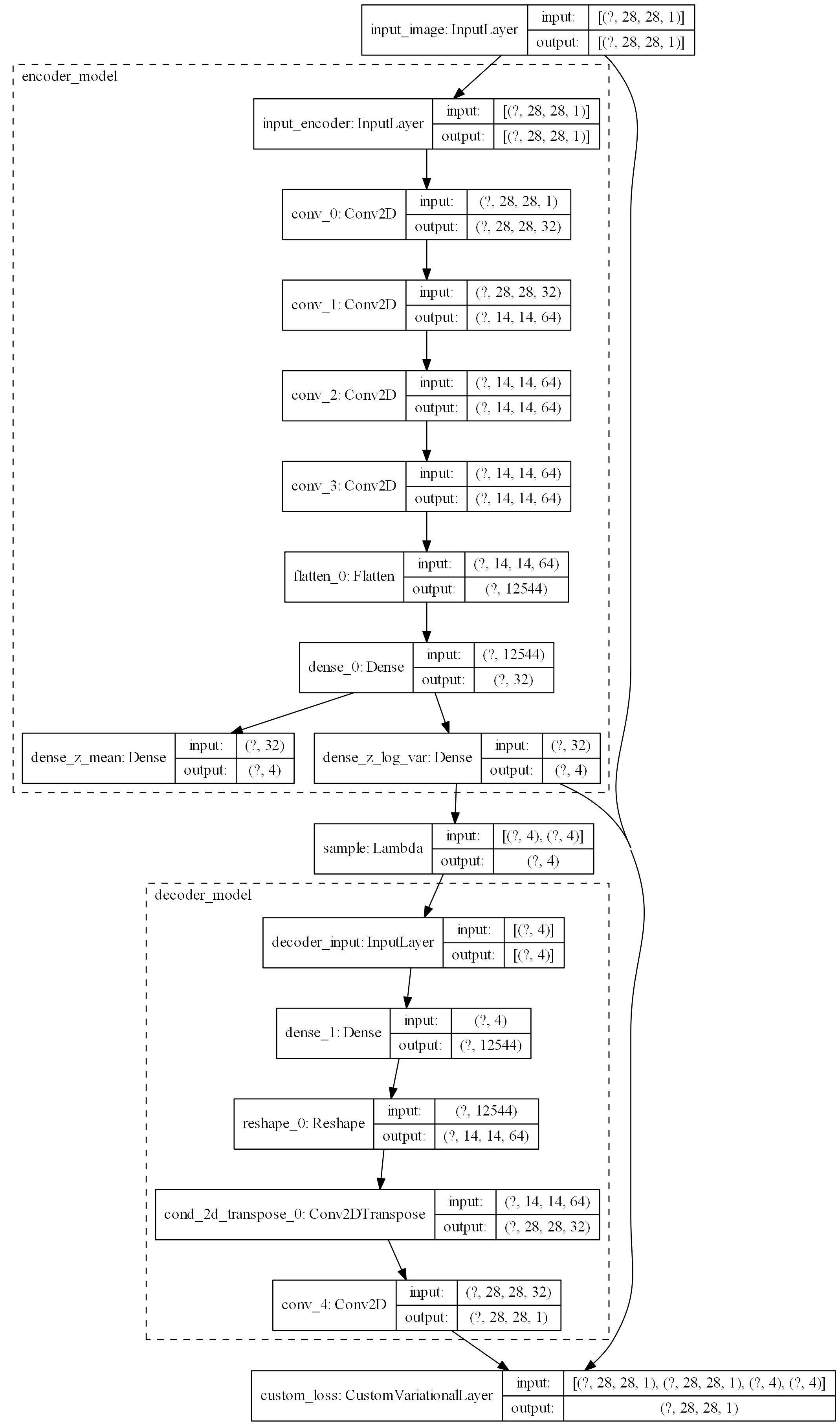
## model plot
tf.keras.utils.plot_model(
vae,
show_shapes=True,
show_layer_names=True,
rankdir='TB',
expand_nested=True,
dpi=50)
Training
We train the data using digit from the MNIST dataset, using only 1 and 8.
(x_train, y_train), (x_test, y_test) = tf.keras.datasets.mnist.load_data()
digit_list = [1, 8]
digit_mask_train = np.isin(y_train, digit_list)
digit_mask_test = np.isin(y_test, digit_list)

x_train = x_train.astype('float32')/255.
x_train = x_train.reshape(x_train.shape + (1,))
x_train = x_train[digit_mask_train,...]

x_test = x_test.astype('float32')/255.
x_test = x_test.reshape(x_test.shape + (1,))
x_test = x_test[digit_mask_test,...]

batch_size = 16
vae.fit(x=x_train, y=None, shuffle=True, epochs=10, batch_size=batch_size, validation_data=(x_test, None))
Final validation losses are about 0.11. We finally save the weights of the trained model:
# vae.save_weights('./weights/weights_1_8.tf', save_format='tf')
vae.load_weights('./weights/weights_1_8.tf')
Intuitions
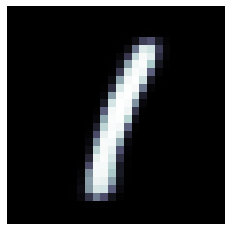
We can now use the trained model to generate new digits, which are not present in the original dataset. Using the latent space vector [0, 1, 0, 0] we obtain a digit similar to a 1:
img = decoder_model.predict(np.array([[0, 1, 0, 0]]))
plt.imshow(np.squeeze(img), cmap=plt.cm.bone)
plt.axis('off')
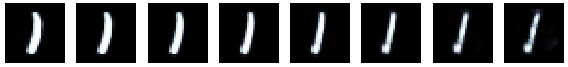
we can explore the latent space by scanning values along a given dimension. For example the first dimension seems to encode information about the thickness of the digit:
fig, axs = plt.subplots(1, 8, figsize=(10, 5))
for ax, latent_variable in zip(axs, np.linspace(-2, 2, axs.size)):
    img_output = decoder_model.predict(np.array([[latent_variable, 1, 1, 1]]))
    ax.imshow(np.squeeze(img_output), cmap='bone')
    ax.set_axis_off()
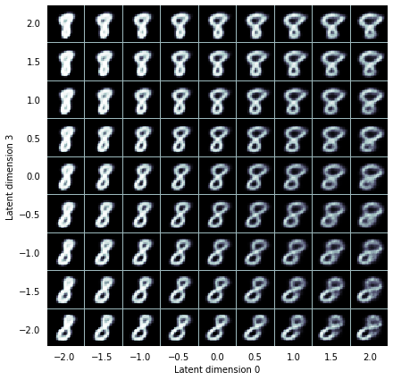
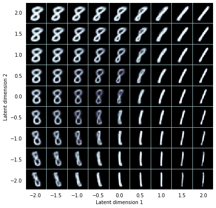
One can explore more direction of the latent space at once, building a 2D grid of output images. If we plot the image generated by scanning the directions 1 and 2 we can see how the first controls how much the digit is bent in the “slash” direction, while the latter how much is bent in the “backslash” direction. The diagonal direction 1-2 controls the transition between the 8 and the 1 digits.
grid_len = 9
img_size = 28
grid = np.ones([(img_size+1)*grid_len-1, (img_size+1)*grid_len-1])*0.7

grid_x = np.linspace(-2, 2, grid_len)
grid_y = np.linspace(-2, 2, grid_len)

for j, latent_0 in enumerate(grid_x):
    for i, latent_1 in enumerate(grid_y):
        z_sample = np.array(np.array([[0, latent_0, latent_1, 0]]))
        x_decoded = decoder_model.predict(z_sample, batch_size=1)[0]
        digit = x_decoded.reshape(img_size, img_size)
        grid[i*img_size+i:(i+1)*img_size+i, j*img_size+j:(j+1)*img_size+j] = digit

fig, ax = plt.subplots(1, figsize=(7, 7))
extent_factor = (grid_len+1)/grid_len
ax.imshow(grid, cmap='bone', extent=np.array([-2, 2, -2, 2])*extent_factor)
ax.set(xticks=np.linspace(-2, 2, grid_len), yticks=np.linspace(-2, 2, grid_len))
ax.set(xlabel='Latent dimension 1', ylabel='Latent dimension 2')
[ax.spines[pos].set_visible(False) for pos in ('right', 'left', 'bottom', 'top')];
[tl.set_color('none') for tl in ax.get_xticklines()];
[tl.set_color('none') for tl in ax.get_yticklines()];
If we instead look at the latent dimensions 0 and 3 in the case of an 8 digit we find out that the first controls the thickness of the digit, while the latter the relative size betweeen the top and the bottom circles forming the eight shape: